| Variable | % Missing | Hypo, N = 2,178 | Non-Hypo, N = 7,016 | Hyper, N = 721 | Non-Hyper, N = 1,459 |
|---|---|---|---|---|---|
| Gender | 0 | ||||
| F | 1,250 (57%) | 4,179 (60%) | 539 (75%) | 1,023 (70%) | |
| M | 928 (43%) | 2,837 (40%) | 182 (25%) | 436 (30%) | |
| Age | 0 | 62 (51, 73) | 64 (53, 76) | 63 (52, 74) | 61 (49, 72) |
| CO2 | 8.6 | 26.0 (24.0, 28.8) | 26.0 (24.0, 29.0) | 26.0 (24.0, 28.0) | 26.0 (24.0, 28.0) |
| CA | 31 | 9.10 (8.50, 9.50) | 9.30 (8.90, 9.60) | 9.40 (9.00, 9.80) | 9.30 (8.80, 9.60) |
| CL | 2.1 | 102.0 (99.0, 104.0) | 101.0 (99.0, 104.0) | 102.0 (99.0, 104.0) | 102.0 (100.0, 105.0) |
| CREA | 0.3 | 1.00 (0.80, 1.30) | 1.00 (0.80, 1.30) | 0.90 (0.70, 1.20) | 0.90 (0.70, 1.10) |
| K | 0.1 | 4.20 (3.90, 4.60) | 4.20 (3.90, 4.60) | 4.20 (3.90, 4.60) | 4.20 (3.90, 4.50) |
| NA | <0.1 | 139.0 (137.0, 141.0) | 139.0 (137.0, 141.0) | 140.0 (137.0, 142.0) | 140.0 (138.0, 142.0) |
| TSH | 0 | 11 (6, 31) | 6 (5, 9) | 0 (0, 0) | 0 (0, 0) |
| BUN | 0.9 | 18 (13, 26) | 19 (14, 25) | 19 (14, 27) | 17 (13, 25) |
| GLU | 31 | 99 (87, 125) | 98 (86, 120) | 101 (88, 131) | 102 (88, 137) |
| HCT | 0 | 35 (30, 39) | 38 (33, 41) | 38 (34, 41) | 38 (33, 41) |
| HGB | <0.1 | 11.50 (9.70, 13.00) | 12.30 (10.70, 13.60) | 12.40 (10.90, 13.50) | 12.30 (10.80, 13.40) |
| PLT | 0.2 | 227 (169, 293) | 236 (180, 298) | 233 (182, 302) | 241 (188, 305) |
| RBC | <0.1 | 3.88 (3.26, 4.40) | 4.11 (3.58, 4.54) | 4.23 (3.73, 4.58) | 4.18 (3.73, 4.56) |
| WBC | <0.1 | 6.8 (5.3, 8.8) | 6.9 (5.5, 8.7) | 7.0 (5.6, 8.8) | 7.2 (5.6, 9.1) |
3 Methods
3.1 IRB
This study was submitted to the Cambell University Institutional Review Board (Campbell IRB) . The study was determined to be Not Human Subjects Research as defined by 45 CFR 46.102(e), and thus exempt from further review by the IRB.
3.2 Population and Data
This study used the Medical Information Mart for Intensive Care (MIMIC) database (Johnson, Alistair et al., n.d.). MIMIC (Medical Information Mart for Intensive Care) is an extensive, freely-available database comprising de-identified health-related data from patients who were admitted to the critical care units of the Beth Israel Deaconess Medical Center. The database contains many different types of information, but only data from the patients and laboratory events table are used in this study. The study uses version IV of the database, comprising data from 2008 - 2019.
3.3 Data Variables and Outcomes
A total of 18 variables were chosen for this study. The age and gender of the patient were pulled from the patient table in the MIMIC database. While this database contains some additional demographic information, it is incomplete and thus unusable for this study. 15 lab values were selected for this study, this includes:
BMP: BUN, bicarbonate, calcium, chloride, creatinine, glucose, potassium, sodium
CBC: Hematocrit, hemoglobin, platelet count, red blood cell count, white blood cell count
TSH
Free T4
The unique patient id and chart time were also retained for identifying each sample. Each sample contains one set of 15 lab values for each patient. Patients may have several samples in the data set run at different times. Rows were retained as long as they had less than three missing results. These missing results can be filled in by imputation later in the process. Samples were also filtered for those with TSH above or below the reference range of 0.27 - 4.2 uIU/mL. These represent samples that would have reflexed for Free T4 testing. After filtering, the final data set contained 11374 rows.
Once the final data set was collected, an additional column was created for the outcome variable to determine if the Free T4 value was diagnostic. This outcome variable was used for building classification models. The classification variable was not used in regression models. Table 3.1 shows how the outcomes were added
| TSH Value | Free T4 Value | Outcome |
|---|---|---|
| >4.2 uIU/ml | >0.93 ng/dL | Non-Hypothyroidism |
| >4.2 uIU/ml | <0.93 ng/dL | Hypothyroidism |
| <0.27 uIU/ml | <1.7 ng/dL | Non-Hyperthyroidism |
| <0.27 uIU/ml | >1.7 ng/dL | Hyperthyroidism |
. Table 3.2 shows the summary statistics of each variable selected for the study. Each numeric variable is listed with the percent missing, median, and interquartile range (IQR). The data set is weighted toward elevated TSH levels, with 80% of values falling into that category. Glucose and Calcium have several missing values at 31 and 31, respectively.
3.4 Data Inspection
By examining Table 3.2 several important data set characteristics quickly come to light without explanation. The median age across the data set, as a whole, is quite similar, with a median age across all categories of 62.5. Females are better represented in the data set, with higher percentages in all categories. Across all categories, the median values for each lab result are pretty similar. The expectation for this is Red Blood cells, which show more considerable variation across the various categories.
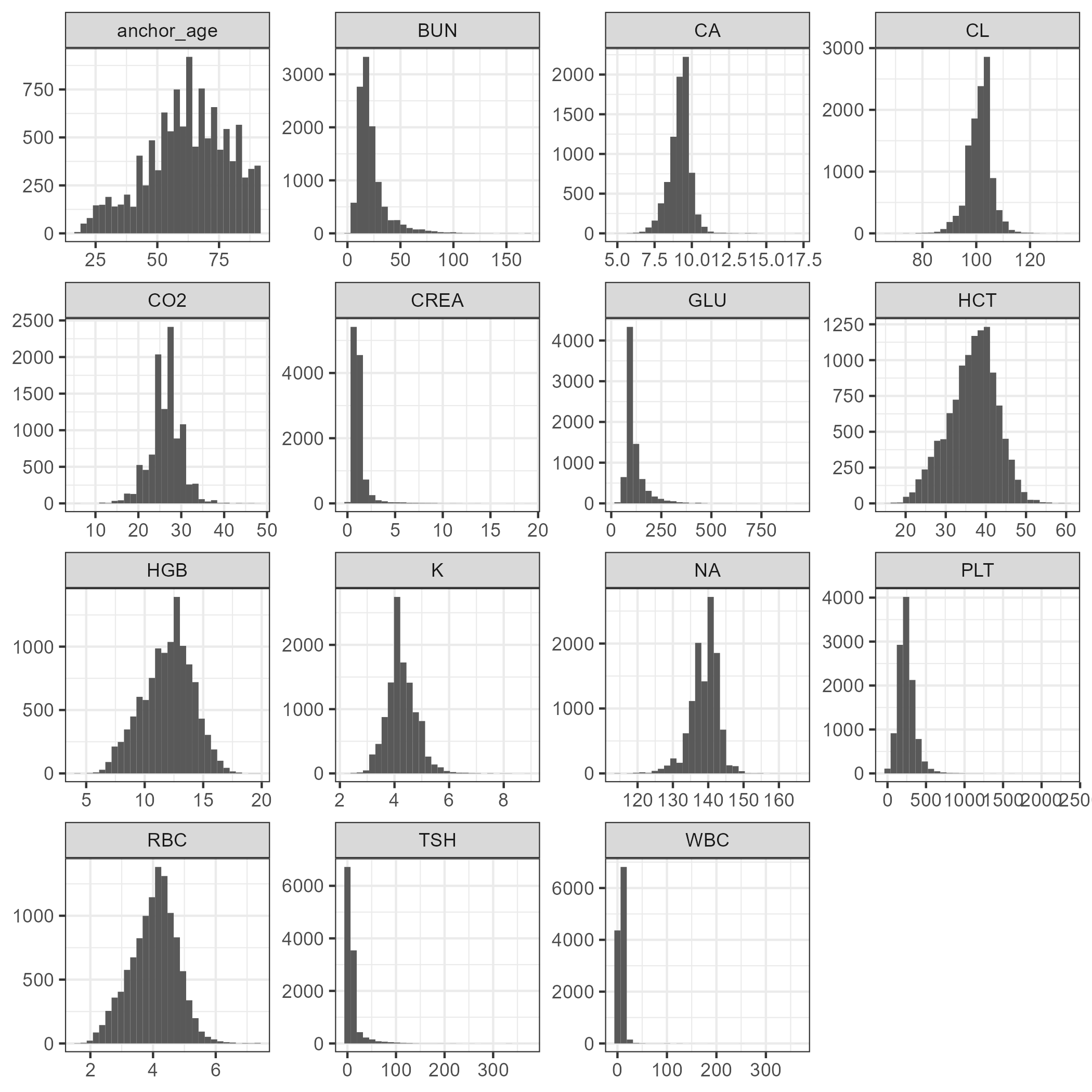
When examining Figure 3.1, many clinical chemistry values do not show a standard distribution. However, the hematology results typically do appear to follow a standard distribution. While not a problem for most tree-based classification models, many regression models perform better with standard variables. Standardizing variables provides a common comparable unit of measure across all the variables (Boehmke & Greenwell, 2020). Since lab values do not contain negative numbers, all numeric values will be log-transformed to bring them to normal distributions.
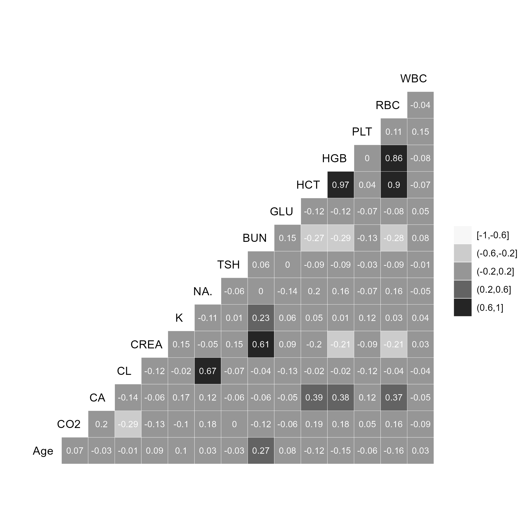
Figure 3.2 shows a high correlation between Hemoglobin, hematocrit, and Red Blood Cell values (as expected). While high correlation does not lead to model issues, it can cause unnecessary computations with little value. However, due to the small number of variables, the computation burden is not expected to cause delays, and thus the variables will not be removed.
3.5 Data Tools
All data handling and modeling were performed using R and R Studio. The current report was rendered in the following environment.
| Setting | Value |
|---|---|
| version | R version 4.2.1 (2022-06-23 ucrt) |
| os | Windows 10 x64 (build 22621) |
| system | x86_64, mingw32 |
| ui | RTerm |
| language | (EN) |
| collate | English_United States.utf8 |
| ctype | English_United States.utf8 |
| tz | America/New_York |
| date | 2023-10-12 |
| pandoc | 3.1.8 @ C:/PROGRA~1/Pandoc/ (via rmarkdown) |
| Package | Loaded Version | Date |
|---|---|---|
| box | 1.1.3 | 2023-05-02 |
| devEMF | 4.4 | 2023-06-14 |
| devtools | 2.4.5 | 2022-10-11 |
| dplyr | 1.1.3 | 2023-09-03 |
| GGally | 2.1.2 | 2021-06-21 |
| ggplot2 | 3.4.2 | 2023-04-03 |
| gtsummary | 1.7.1 | 2023-04-27 |
| here | 1.0.1 | 2020-12-13 |
| knitr | 1.43 | 2023-05-25 |
| magrittr | 2.0.3 | 2022-03-30 |
| readr | 2.1.3 | 2022-10-01 |
| rmarkdown | 2.22 | 2023-06-01 |
| tibble | 3.2.1 | 2023-03-20 |
| tidyr | 1.3.0 | 2023-01-24 |
3.6 Model Selection
Both classification and regression models were screened using a random grid search to tune hyperparameters. The models were tested against the training data set to find the best-fit model. Figure 3.3 shows the results of the model screening for regression models, using root mean square error (RMSE) as the ranking method. Random Forest models and boosted trees performed similarly and were selected for further testing. A full grid search was performed on both models, with a Random Forest model as the final selection. The final hyperparameters selected were:
mtry: 8
trees: 1000
minimum nodes: 2

Figure 3.4 shows the results of the model screen for classification models using accuracy as the ranking method. As with regression models, boosted trees and random forest models performed the best. After completing a full grid search of both model types, a random forest model was again chosen as the final model. The final hyperparameters for the model selected were:
mtry: 8
trees: 2000
minimum nodes: 2
